Adaptive Subdivision of Bezier Curves
An attempt to achieve perfect result in Bezier curve approximation

First published in July, 2005

Bezier curves are widely used in modern 2D and 3D graphics. In most applications it's quite enough to use only quadric and cubic curves. There is a huge number of explanations in the Internet about Bezier curves and I believe if you read it you know the topic. The main question is is how we can actually draw the curve.

It's a common practice that the curves are approximated with a number of short line segments and it's the only efficient way to draw them. In this article I will try to explain a method of almost perfect approximation keeping the minimal number of points.

First of all, we have a look at the very basic method Paul Bourke described here:
http://astronomy.swin.edu.au/~pbourke/curves/bezier

Below is a piece of code for calculation of the arbitrary point of a cubic curve (an exact copy from Paul's web-site):

/*
   Four control point Bezier interpolation
   mu ranges from 0 to 1, start to end of curve
*/
XYZ Bezier4(XYZ p1,XYZ p2,XYZ p3,XYZ p4,double mu)
{
   double mum1,mum13,mu3;
   XYZ p;

   mum1 = 1 - mu;
   mum13 = mum1 * mum1 * mum1;
   mu3 = mu * mu * mu;

   p.x = mum13*p1.x + 3*mu*mum1*mum1*p2.x + 3*mu*mu*mum1*p3.x + mu3*p4.x;
   p.y = mum13*p1.y + 3*mu*mum1*mum1*p2.y + 3*mu*mu*mum1*p3.y + mu3*p4.y;
   p.z = mum13*p1.z + 3*mu*mum1*mum1*p2.z + 3*mu*mu*mum1*p3.z + mu3*p4.z;

   return(p);
}

Here we have four control points and parameter “mu” in range from 0 to 1. Technically that's enough. We simply calculate a number of points with increasing “mu” and draw straight line segments between them.

First of all, the method is expensive; each point in 2D requires 24 multiplicatoins with floating point. But this problem can be easily solved if we replace direct calculations by an incremental (recurrent) method. It's described here: Interpolation with Bezier Curves, at the end of the article. As you can see, the main loop contains only six addition operations. And as far as I know this is the fastest method, especially on modern processors, where floating point operations are quite fast.

But the main problem is how to determine the number of points itself and how to increase that very “mu”. The simplest method is to select a certain step, say, 0.01, so that, any curve will be divided into 99 straight line segments. The disadvantage is obvious, long curves will have too few points, short ones — to many of them.

Apparently, we need to calculate the step on the basis of the length of the curve. To do that we need to calculate the actual length of the curve, but to calculate the length we need to calculate the curve itself. It's a classical “catch 22” situation. A rather good estimation is the sum of the distances:

(p1,p2)+(p2,p3)+(p3,p4);

So that, experimentally I found out that for typical screen resolutions it's good enough to have the following estimation:

    dx1 = x2 - x1;
    dy1 = y2 - y1;
    dx2 = x3 - x2;
    dy2 = y3 - y2;
    dx3 = x4 - x3;
    dy3 = y4 - y3;

    len = sqrt(dx1 * dx1 + dy1 * dy1) + 
          sqrt(dx2 * dx2 + dy2 * dy2) + 
          sqrt(dx3 * dx3 + dy3 * dy3);

    num_steps = int(len * 0.25);

Note that we are talking in terms of Anti-Aliasing and Subpixel Accuracy. It makes a huge difference compared with regular pixel accuracy MoveTo/LineTo interface.

But even if we estimate the curve step accurately the problems still persist. A cubic curve can have rather sharp turns, narrow loops or even cusps. Look at the following picture:

Here we have a curve approximated with 52 line segments. But still, after drawing an equidistant outine (stroke) the loop looks rather inaccurate. To achieve good accuracy we have to increase the number of points:

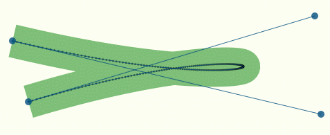Here we have 210 line segments and it's clearly seen that most of them are useless. In other words it produces too many points at “flat” parts of the curve and too few of them at sharp turns.

But even if we have a tiny step we still have problems:

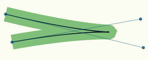This curve is approximated with 1091 line segments (sic!), but still fails at a sharp turn (almost a cusp).

Ideally we would want to have an adaptive step. Look at the following picture:

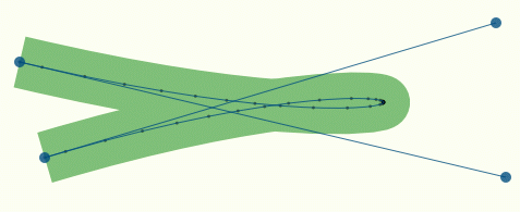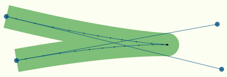
It has only 40 line segments, but almost perfectly approximates the curve, considering its outline (stroke). This is the result we really want to achieve and it really is achieved. Note that even with very sharp turns the stroke remains smooth and the number of line segments is quite reasonable; in this case it's only 44:

Paul de Casteljau, a brilliant engineer at Citroen discovered a very interesting property of any Bezier curve. It's namely that any curve of any degree can be easily divided into two curves of the same degree. The following picture is classical:

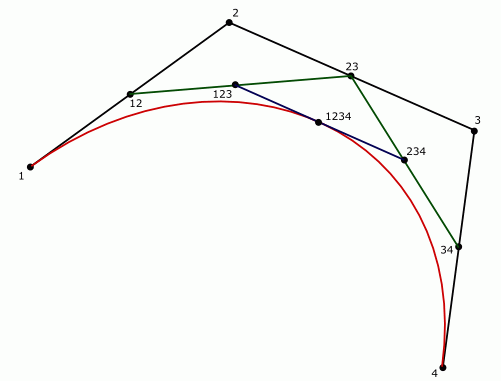Here we have control points 1,2,3,4. Then we calculate midpoints 12,23,34, then midpoints 123 and 234, and finally point 1234 lying on the curve. Instead of midpoint (coefficient 0.5) there can be any other coefficient from 0 to 1, but in this article we use namely midpoints. The two new curves exactly coincide with the original ones and they are defined by points: 1,12,123,1234 (the left one) and 1234,234,34,4 (the right one).

It's clearly seen that the new curves are more “flat” than the original one, so, if we repeat the operation a certain numbrer of times we can simply replace the curve with a line segment.

The recursive program code of subdivision is also classical:

void recursive_bezier(double x1, double y1, 
                      double x2, double y2, 
                      double x3, double y3, 
                      double x4, double y4)
{
    // Calculate all the mid-points of the line segments
    //----------------------
    double x12   = (x1 + x2) / 2;
    double y12   = (y1 + y2) / 2;
    double x23   = (x2 + x3) / 2;
    double y23   = (y2 + y3) / 2;
    double x34   = (x3 + x4) / 2;
    double y34   = (y3 + y4) / 2;
    double x123  = (x12 + x23) / 2;
    double y123  = (y12 + y23) / 2;
    double x234  = (x23 + x34) / 2;
    double y234  = (y23 + y34) / 2;
    double x1234 = (x123 + x234) / 2;
    double y1234 = (y123 + y234) / 2;

    if(curve_is_flat)
    {
        // Draw and stop
        //----------------------
        draw_line(x1, y1, x4, y4);
    }
    else
    {
        // Continue subdivision
        //----------------------
        recursive_bezier(x1, y1, x12, y12, x123, y123, x1234, y1234); 
        recursive_bezier(x1234, y1234, x234, y234, x34, y34, x4, y4); 
    }
}

That's that! It's all you need to draw a cubic Bezier curve. But the devil is in the condition “curve_is_flat”.

The Casteljau's subdivision method has a great advantage. Really, we can estimate the flatness of the curve because we have information about it — the initial control points plus all other intermediate points. In case of the incremental method all we have is just a point. Well, of course we can take at least two points before and analyze them, but it will complicate the whole thing a lot.

There can be many criteria of when to stop subdivision. You can calculate the distance between points 1 and 4 in the simplest case. It's a bad criterion because initially points 1 and 4 may coincide. Well, there is a workaround, namely that we force the subdivision the first time.

A better condition would be to calculate the distance between a point and a line. It's proportional to the actual error of approximation. The main question is what distances we should consider.

Initially I thought that the distance between point 1234 and line (1-4) is enough. It can be zero in a "Z" case, for example, (100, 100, 200, 100, 100, 200, 200, 200).

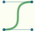But this sutuation is solved by forcing the subdivision the first time.

But after conducting of many experiments I found out that the sum of 3 distances works much better:

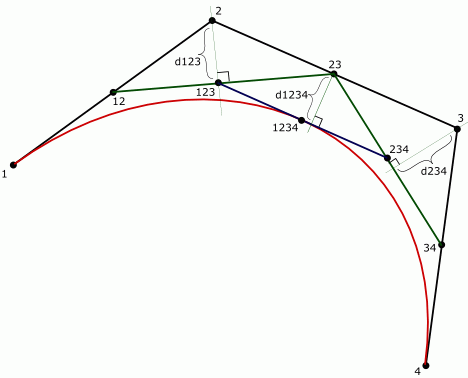Here we sum three distances: d123+d1234+d234. This criterion doesn't require forcing the first subdivision.

Then, after having even more experiments I discivered that the criterion with two distances works even better and it doesn't require forcing the first subdivision either. It's the sum of the distances d2+d3:

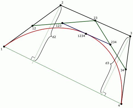That's it, we have a rather good estimation of the approximation error. Calculation of the distance between a point and a line can seem expensive, but it isn't. We don't even have to calculate square roots! Remember, all we need is just to estimate and compare the error (yes/no).

So that, the program code is as follows:

    void recursive_bezier(double x1, double y1, 
                          double x2, double y2, 
                          double x3, double y3, 
                          double x4, double y4)
    {

        // Calculate all the mid-points of the line segments
        //----------------------
        double x12   = (x1 + x2) / 2;
        double y12   = (y1 + y2) / 2;
        double x23   = (x2 + x3) / 2;
        double y23   = (y2 + y3) / 2;
        double x34   = (x3 + x4) / 2;
        double y34   = (y3 + y4) / 2;
        double x123  = (x12 + x23) / 2;
        double y123  = (y12 + y23) / 2;
        double x234  = (x23 + x34) / 2;
        double y234  = (y23 + y34) / 2;
        double x1234 = (x123 + x234) / 2;
        double y1234 = (y123 + y234) / 2;

        // Try to approximate the full cubic curve by a single straight line
        //------------------
        double dx = x4-x1;
        double dy = y4-y1;

        double d2 = fabs(((x2 - x4) * dy - (y2 - y4) * dx));
        double d3 = fabs(((x3 - x4) * dy - (y3 - y4) * dx));

        if((d2 + d3)*(d2 + d3) < m_distance_tolerance * (dx*dx + dy*dy))
        {
            add_point(x1234, y1234);
            return;
        }

        // Continue subdivision
        //----------------------
        recursive_bezier(x1, y1, x12, y12, x123, y123, x1234, y1234); 
        recursive_bezier(x1234, y1234, x234, y234, x34, y34, x4, y4); 
    }


    void bezier(double x1, double y1, 
                double x2, double y2, 
                double x3, double y3, 
                double x4, double y4)
    {
        add_point(x1, y1);
        recursive_bezier(x1, y1, x2, y2, x3, y3, x4, y4);
        add_point(x4, y4);
    }

Where m_distance_tolerance is the square of the maximal distance you can afford. In typical screen resolution it's normally about 0.5*0.5 = 0.25

That's it, we have solved the task of having the minimal number of points with constant maximal error along the entire curve. Note that the incremental method produces much more points, but the approximation error at flat parts is too little (no necessary to divide the curve into so many number of points), while the one at sharp turns is too high. The subdivision method minimizes the number of points keeping the maximal approximation error about a constant.

But this methods has more serious problems. If points 1 and 4 coincide, both values, (d2 + d3)*(d2 + d3) and (dx*dx + dy*dy) will be strictly zero. It's one of the rear cases when comparoson "Less" and "LessEqual" makes difference in floating point. The division will continue in this case, and if the condition is "LessEqual" it will stop. But this code will result in stack overflow in cases when 3 or all 4 points coincide. We could solve it using "LessEqual" in the condition and forcing the first subdivision. But more careful analysis showed that it won't help. After one subdivision one of the "subcurves" can still have a loop and in particular, coinciding endpoints. All these difficulties will be overcome later, but first let's talk about estimation by angle.

The code above solves the task of optimization of the number of points keeping the approximation error about a constant along the entire curve. But it has the same problem as the incremental method at sharp turns:

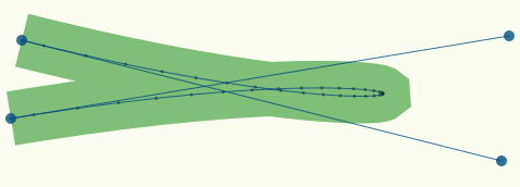This approximation has 36 line segments and the maximal error of 0.08 pixel.

Obviously using only estimation by distance is not enough. To keep wide strokes smooth with any conditions we should estimate the curvature by angle, regardless of the actual lengths or distances.

When subdividing, the two new curves are more flat than the initial one. It also means that the tangents at the start and at the end (points 1 and 4) are about the same. If they are considerably different the curve has a sharp turn at that point, so that, we should continue subdivision.

So that, we introduce another criterion, m_angle_tolerance:

    // If the curvature doesn't exceed the distance_tolerance value
    // we tend to finish subdivisions.
    //----------------------
    if(m_angle_tolerance < curve_angle_tolerance_epsilon)
    {
        m_points.add(point_type(x1234, y1234));
        return;
    }

    // Angle & Cusp Condition
    //----------------------
    double a23 = atan2(y3 - y2, x3 - x2);
    double da1 = fabs(a23 - atan2(y2 - y1, x2 - x1));
    double da2 = fabs(atan2(y4 - y3, x4 - x3) - a23);
    if(da1 >= pi) da1 = 2*pi - da1;
    if(da2 >= pi) da2 = 2*pi - da2;

    if(da1 + da2 < m_angle_tolerance)
    {
        // Finally we can stop the recursion
        //----------------------
        m_points.add(point_type(x1234, y1234));
        return;
    }

Here we use m_angle_tolerance also as a flag. If its value is less than a certain epsion we do not process angles at all.

The following picture illustrates the calculations:

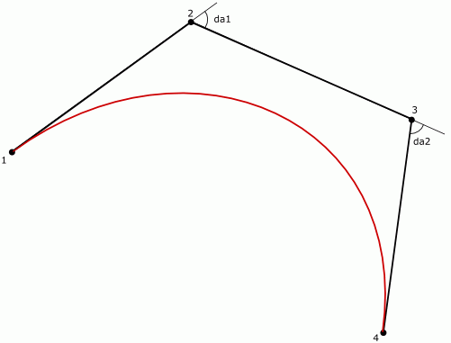Well, technically it would be enough to calculate just one angle between the first and the third line segments (1-2 and 3-4) but the two angles will be useful later, when we process the cusps.

This code guarantees that any two consecutive line segments will be flat enough to calculate smoothly looking strokes. But it has problems too, and first of all it's processing of the cusps.

A cubic curve can have a cusp. A cusp is a point on the curve at which curve tangent is discontinuous. It's a sharp turn that remains sharp no matter how much you zoom it in. In other words there is no way that fat mitter-join stroke can ever look as turning smoothly around that point. Tangent is discontinuous so stroke should display sharp turn as well.

To have a real cusp the control points should be exactly of the form of letter "X", for example:

(100, 100, 300, 200, 200, 200, 200, 100)

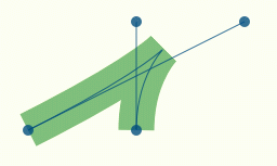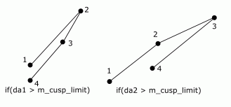
In this case condition da1 + da2 < m_angle_tolerance will never theoretically occur. In practice it will occur as soon as all 4 control points exactly coincide and all the arguments of all calls to atan2() will be strictly zero. But when it happens the recursion will very very deep and you can even have stack overflow. Thet's the bad news. The good news is that it has a very simple workaround:

    if(da1 > m_cusp_limit)
    {
        m_points.add(point_type(x2, y2));
        return;
    }

    if(da2 > m_cusp_limit)
    {
        m_points.add(point_type(x3, y3));
        return;
    }

Note that we usually add point 1234 that lies on the curve. That's because it allows us to distribute the points symmetrically with regard to the endpoints. But here we add the point at wich we have a sharp angle. I came up with this idea after some experimets. It ensures that the cut of the stroke will be perpendicular to the lines at the cusp.

But it all is not enough! There is a lot of different degenerate cases when this algorithm fails. And it took me pretty long time to analyze it and to compose something that shoots all the cases with one silver bullet. It would be huge amount of code to consider all cases separately and I hate spaghetti-code. For example, points can coincide and in this case calculations of the angles fail. You see, in case of uncertainty, function atan2(0,0) returns zero, as if the line was horizontal. I will skip all my “throes of composition” and just give you the bottom line.

As my experiments showed all the bad cases can be treated as colliner ones.

To esimate the distance we calculate the following expressions:

    double dx = x4-x1;
    double dy = y4-y1;
    double d2 = fabs(((x2 - x4) * dy - (y2 - y4) * dx));
    double d3 = fabs(((x3 - x4) * dy - (y3 - y4) * dx));

Then, if we divide d2 by the length of line segment 1-4 we will have the distance between point 2 and the line 1-4. But as it was mentioned above we don't need to have a real distance, we only need to compare it. In particular it means that we can also filter the coinciding points and all other collinear cases if we introduce some value of curve_collinearity_epsilon:

    double dx = x4-x1;
    double dy = y4-y1;

    double d2 = fabs(((x2 - x4) * dy - (y2 - y4) * dx));
    double d3 = fabs(((x3 - x4) * dy - (y3 - y4) * dx));

    if(d2 > curve_collinearity_epsilon && d3 > curve_collinearity_epsilon)
    { 
        // Regular care
        . . .
    }
    else
    {
        if(d2 > curve_collinearity_epsilon)
        {
            // p1,p3,p4 are collinear (or coincide), p2 is considerable
            . . .
        }
        else
        if(d3 > curve_collinearity_epsilon)
        {
            // p1,p2,p4 are collinear (or coincide), p3 is considerable
            . . .
        }
        else
        {
            // Collinear case
            . . .
        }
    }

In the collinear (or coinciding points) cases we can do differently. And one of the cases is when all four points are collinear. The most amazing thing is that the collinearity check perfectly protects us from very deep recursion in cases when we have real cusps. We can do without limiting the cusps and can remove the code that controls the cusp limit. But I still left it as is with an additional condition of whether we should limit cusps or not. Just because in some cases it can be useful.

I would like to thank Timothee Groleau, http://www.timotheegroleau.com for the great and simple idea of estimation of the momentary curvature. It's simply the distance between point 1234 and the midpoint of 1-4. It's totally different from estimating of the distance between a point and a line. His method also gives us quite appropriate result, although it's still generally worse. But it has a very important advantage. It handles the collinear case, when the control points have the following order:

2--------1---------4----------3

Any method with the criterion of line-point distance will fail in this case. There will be just one line segment 1-4, which is obviously wrong. Timothee's criterion works well in this case and we already have a mechanism of detecting the collinearity! So that, the code of handling the collinear case is pretty simple:

    . . .
    else
    {
        // Collinear case
        //-----------------
        dx = x1234 - (x1 + x4) / 2;
        dy = y1234 - (y1 + y4) / 2;
        if(dx*dx + dy*dy <= m_distance_tolerance)
        {
            m_points.add(point_type(x1234, y1234));
            return;
        }
    }

The only thing we need to do is to enforce subdivision one time, because There can be a "Z" case mentioned above.

So that, the pseudo-code looks as follows:

void recursive_bezier(double x1, double y1, 
                      double x2, double y2, 
                      double x3, double y3, 
                      double x4, double y4,
                      unsigned level)
{
    double x12   = (x1 + x2) / 2;
    double y12   = (y1 + y2) / 2;
    double x23   = (x2 + x3) / 2;
    double y23   = (y2 + y3) / 2;
    double x34   = (x3 + x4) / 2;
    double y34   = (y3 + y4) / 2;
    double x123  = (x12 + x23) / 2;
    double y123  = (y12 + y23) / 2;
    double x234  = (x23 + x34) / 2;
    double y234  = (y23 + y34) / 2;
    double x1234 = (x123 + x234) / 2;
    double y1234 = (y123 + y234) / 2;

    if(level)
    {
        if(curve_is_flat)
        {
            draw_line(x1, y1, x4, y4);
            return;
        }
    }

    recursive_bezier(x1, y1, x12, y12, x123, y123, x1234, y1234, level + 1); 
    recursive_bezier(x1234, y1234, x234, y234, x34, y34, x4, y4, level + 1); 
}

It also allows us to limit the recursion. Well, it seems that we don't have to limit it (it's already limited by the other criteria), but the strict mathematical proof of it is extremally difficult to me, so, just in case I limit the recursion by 32. In practice I have never seen deeper than 17 with extremally hard conditions (very long curve, thousands of points, tiny error, plus a cusp).

Timothee's criterion produces a number of points when we have another collinear case: 1---2---3-------4. It would be good to detect it too and to produce only two points (1-4), but I think it's not that important because the cases of strict collinearity are very rear. So, in practice it won't affect the performance anyhow.

There are two other cases of collinearity:

    if(d2 > curve_collinearity_epsilon)
    {
        // p1,p3,p4 are collinear (or coincide), p2 is considerable
        . . .
    }
    else
    if(d3 > curve_collinearity_epsilon)
    {
        // p1,p2,p4 are collinear (or coincide), p3 is considerable
        . . .
    }

That's easy. We simply treat points 1 and 3 as coinciding (points 2 and 4 in the second case). Well, there is still one detail that I'll tell you about.

Finally we can publish the full source code.

    //------------------------------------------------------------------------
    void curve4_div::init(double x1, double y1, 
                          double x2, double y2, 
                          double x3, double y3,
                          double x4, double y4)
    {
        m_points.remove_all();
        m_distance_tolerance = 0.5 / m_approximation_scale;
        m_distance_tolerance *= m_distance_tolerance;
        bezier(x1, y1, x2, y2, x3, y3, x4, y4);
        m_count = 0;
    }

    //------------------------------------------------------------------------
    void curve4_div::recursive_bezier(double x1, double y1, 
                                      double x2, double y2, 
                                      double x3, double y3, 
                                      double x4, double y4,
                                      unsigned level)
    {
        if(level > curve_recursion_limit) 
        {
            return;
        }

        // Calculate all the mid-points of the line segments
        //----------------------
        double x12   = (x1 + x2) / 2;
        double y12   = (y1 + y2) / 2;
        double x23   = (x2 + x3) / 2;
        double y23   = (y2 + y3) / 2;
        double x34   = (x3 + x4) / 2;
        double y34   = (y3 + y4) / 2;
        double x123  = (x12 + x23) / 2;
        double y123  = (y12 + y23) / 2;
        double x234  = (x23 + x34) / 2;
        double y234  = (y23 + y34) / 2;
        double x1234 = (x123 + x234) / 2;
        double y1234 = (y123 + y234) / 2;

        if(level > 0) // Enforce subdivision first time
        {
            // Try to approximate the full cubic curve by a single straight line
            //------------------
            double dx = x4-x1;
            double dy = y4-y1;

            double d2 = fabs(((x2 - x4) * dy - (y2 - y4) * dx));
            double d3 = fabs(((x3 - x4) * dy - (y3 - y4) * dx));

            double da1, da2;

            if(d2 > curve_collinearity_epsilon && d3 > curve_collinearity_epsilon)
            { 
                // Regular care
                //-----------------
                if((d2 + d3)*(d2 + d3) <= m_distance_tolerance * (dx*dx + dy*dy))
                {
                    // If the curvature doesn't exceed the distance_tolerance value
                    // we tend to finish subdivisions.
                    //----------------------
                    if(m_angle_tolerance < curve_angle_tolerance_epsilon)
                    {
                        m_points.add(point_type(x1234, y1234));
                        return;
                    }

                    // Angle & Cusp Condition
                    //----------------------
                    double a23 = atan2(y3 - y2, x3 - x2);
                    da1 = fabs(a23 - atan2(y2 - y1, x2 - x1));
                    da2 = fabs(atan2(y4 - y3, x4 - x3) - a23);
                    if(da1 >= pi) da1 = 2*pi - da1;
                    if(da2 >= pi) da2 = 2*pi - da2;

                    if(da1 + da2 < m_angle_tolerance)
                    {
                        // Finally we can stop the recursion
                        //----------------------
                        m_points.add(point_type(x1234, y1234));
                        return;
                    }

                    if(m_cusp_limit != 0.0)
                    {
                        if(da1 > m_cusp_limit)
                        {
                            m_points.add(point_type(x2, y2));
                            return;
                        }

                        if(da2 > m_cusp_limit)
                        {
                            m_points.add(point_type(x3, y3));
                            return;
                        }
                    }
                }
            }
            else
            {
                if(d2 > curve_collinearity_epsilon)
                {
                    // p1,p3,p4 are collinear, p2 is considerable
                    //----------------------
                    if(d2 * d2 <= m_distance_tolerance * (dx*dx + dy*dy))
                    {
                        if(m_angle_tolerance < curve_angle_tolerance_epsilon)
                        {
                            m_points.add(point_type(x1234, y1234));
                            return;
                        }

                        // Angle Condition
                        //----------------------
                        da1 = fabs(atan2(y3 - y2, x3 - x2) - atan2(y2 - y1, x2 - x1));
                        if(da1 >= pi) da1 = 2*pi - da1;

                        if(da1 < m_angle_tolerance)
                        {
                            m_points.add(point_type(x2, y2));
                            m_points.add(point_type(x3, y3));
                            return;
                        }

                        if(m_cusp_limit != 0.0)
                        {
                            if(da1 > m_cusp_limit)
                            {
                                m_points.add(point_type(x2, y2));
                                return;
                            }
                        }
                    }
                }
                else
                if(d3 > curve_collinearity_epsilon)
                {
                    // p1,p2,p4 are collinear, p3 is considerable
                    //----------------------
                    if(d3 * d3 <= m_distance_tolerance * (dx*dx + dy*dy))
                    {
                        if(m_angle_tolerance < curve_angle_tolerance_epsilon)
                        {
                            m_points.add(point_type(x1234, y1234));
                            return;
                        }

                        // Angle Condition
                        //----------------------
                        da1 = fabs(atan2(y4 - y3, x4 - x3) - atan2(y3 - y2, x3 - x2));
                        if(da1 >= pi) da1 = 2*pi - da1;

                        if(da1 < m_angle_tolerance)
                        {
                            m_points.add(point_type(x2, y2));
                            m_points.add(point_type(x3, y3));
                            return;
                        }

                        if(m_cusp_limit != 0.0)
                        {
                            if(da1 > m_cusp_limit)
                            {
                                m_points.add(point_type(x3, y3));
                                return;
                            }
                        }
                    }
                }
                else
                {
                    // Collinear case
                    //-----------------
                    dx = x1234 - (x1 + x4) / 2;
                    dy = y1234 - (y1 + y4) / 2;
                    if(dx*dx + dy*dy <= m_distance_tolerance)
                    {
                        m_points.add(point_type(x1234, y1234));
                        return;
                    }
                }
            }
        }

        // Continue subdivision
        //----------------------
        recursive_bezier(x1, y1, x12, y12, x123, y123, x1234, y1234, level + 1); 
        recursive_bezier(x1234, y1234, x234, y234, x34, y34, x4, y4, level + 1); 
    }

    //------------------------------------------------------------------------
    void curve4_div::bezier(double x1, double y1, 
                            double x2, double y2, 
                            double x3, double y3, 
                            double x4, double y4)
    {
        m_points.add(point_type(x1, y1));
        recursive_bezier(x1, y1, x2, y2, x3, y3, x4, y4, 0);
        m_points.add(point_type(x4, y4));
    }

It's not full to be honest, but it shows the algorithm. The rest (class definition) can be found here:

Class curve4_div, files agg_curves.h, agg_curves.cpp.

The detail I was talking about is the following piece of code when processing the collinear cases:

    if(da1 < m_angle_tolerance)
    {
        m_points.add(point_type(x2, y2));
        m_points.add(point_type(x3, y3));
        return;
    }

You see, here we also add two points, instead of one (1234). I came up with this also experimentally. Adding just one point (any of them) produces wrong cut at the cusp (wrong angle). I'm not quite sure about the mathematical meaning of it, but… it just works!

The class has the following parameters:

• approximation_scale — Eventually determines the approximation accuracy. In practice we need to transform points from the World coordinate system to the Screen one. It always has some scaling coefficient. The curves are usually processed in the World coordinates, while the approximation accuracy should be eventually in pixels. Usually it looks as follows:
  m_curved.approximation_scale(m_transform.scale()); where m_transform is the affine matrix that includes all the transformations, including viewport and zoom.
• angle_tolerance — You set it in radians. The less this value is the more accurate will be the approximation at sharp turns. But 0 means that we don't consider angle conditions at all.
• cusp_limit — An angle in radians. If 0, only the real cusps will have bevel cuts. If more than 0, it will restrict the sharpness. The more this value is the less sharp turns will be cut. Typically it should not exceed 10-15 degrees.

As I mentioned above estimation by angles is expensive and we not always need it. We need it only in cases of considerable strokes or contours of the curves. To optimize it we can do approximately the following:

    double scl = m_transform.scale();
    m_curved.approximation_scale(scl);

    // Turn off processing of curve cusps
    //-----------------
    m_curved.angle_tolerance(0);

    if(attr.fill_flag)
    {
        // Process the fill
        . . .
    }

    if(attr.stroke_flag)
    {
        // Process the stroke
        //---------------------
        // If the *visual* line width is considerable we 
        // turn on processing of sharp turns and cusps.
        //---------------------
        if(attr.stroke_width * scl > 1.0)
        {
            m_curved.angle_tolerance(0.2);
        }
        . . .
    }

It considerably speeds up the overall processing.

Quadric curves are much simpler to handle. We don't even need the cusp_limit creiterion because the collinearity check handles all the degenerate cases.

    //------------------------------------------------------------------------
    void curve3_div::init(double x1, double y1, 
                          double x2, double y2, 
                          double x3, double y3)
    {
        m_points.remove_all();
        m_distance_tolerance = 0.5 / m_approximation_scale;
        m_distance_tolerance *= m_distance_tolerance;
        bezier(x1, y1, x2, y2, x3, y3);
        m_count = 0;
    }


    //------------------------------------------------------------------------
    void curve3_div::recursive_bezier(double x1, double y1, 
                                      double x2, double y2, 
                                      double x3, double y3,
                                      unsigned level)
    {
        if(level > curve_recursion_limit) 
        {
            return;
        }

        // Calculate all the mid-points of the line segments
        //----------------------
        double x12   = (x1 + x2) / 2;                
        double y12   = (y1 + y2) / 2;
        double x23   = (x2 + x3) / 2;
        double y23   = (y2 + y3) / 2;
        double x123  = (x12 + x23) / 2;
        double y123  = (y12 + y23) / 2;

        double dx = x3-x1;
        double dy = y3-y1;
        double d = fabs(((x2 - x3) * dy - (y2 - y3) * dx));

        if(d > curve_collinearity_epsilon)
        { 
            // Regular care
            //-----------------
            if(d * d <= m_distance_tolerance * (dx*dx + dy*dy))
            {
                // If the curvature doesn't exceed the distance_tolerance value
                // we tend to finish subdivisions.
                //----------------------
                if(m_angle_tolerance < curve_angle_tolerance_epsilon)
                {
                    m_points.add(point_type(x123, y123));
                    return;
                }

                // Angle & Cusp Condition
                //----------------------
                double da = fabs(atan2(y3 - y2, x3 - x2) - atan2(y2 - y1, x2 - x1));
                if(da >= pi) da = 2*pi - da;

                if(da < m_angle_tolerance)
                {
                    // Finally we can stop the recursion
                    //----------------------
                    m_points.add(point_type(x123, y123));
                    return;                 
                }
            }
        }
        else
        {
            // Collinear case
            //-----------------
            dx = x123 - (x1 + x3) / 2;
            dy = y123 - (y1 + y3) / 2;
            if(dx*dx + dy*dy <= m_distance_tolerance)
            {
                m_points.add(point_type(x123, y123));
                return;
            }
        }

        // Continue subdivision
        //----------------------
        recursive_bezier(x1, y1, x12, y12, x123, y123, level + 1); 
        recursive_bezier(x123, y123, x23, y23, x3, y3, level + 1); 
    }

    //------------------------------------------------------------------------
    void curve3_div::bezier(double x1, double y1, 
                            double x2, double y2, 
                            double x3, double y3)
    {
        m_points.add(point_type(x1, y1));
        recursive_bezier(x1, y1, x2, y2, x3, y3, 0);
        m_points.add(point_type(x3, y3));
    }

You can doanload a demo appication for Win32 from here.

Below is the screenshot:

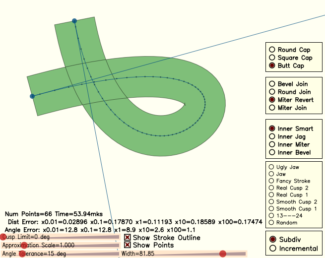It works rather slow, but it's not a concern. I calculate the maximal distance and angle error for five scales: 0.01, 0.1, 1, 10, and 100 (which is rather time consuming). The distance error means that we set the approximation_scale() to the one of the above values, calculate the maximal deviation and then multiply it by the approximation_scale() value. So that, it will be the maximal error normalized to the screen resolution (pixels).

The reference curve is calculated using the direct method Paul Bourke describes (see Introduction) with a very little step (4096 points).

You can clearly see the difference in the maximal deviation in the incremental and subdivision methods. In the subdivision method the maximal error remains about the same regardless of the scale (or decreases on scales 0.01 and 0.1). But in the incremental method it decreases on the 10x and 100x scales. This behaviour is apparently wrong because we don't need the error of 0.001 pixel. It means that the curve has too many points. We need to keep a balance of the error and the number of points.

You can also compare the results of rendering:
Incremental Tiger
Subdivided Tiger

The difference is seems to be very litte, but if you download these pictures and switch between them in some slideshow program you will see it. In these examples I tried to set the approximation accuracy in such a way that the eventual number of vertices would be about the same (I even gave the incremental method some extra allowance). If you carefully compare the pictures you will see that the subdivision method gives us much more accurate result.

Still, the incremental method is also nice. It's simple and fast and can be used in cases when the performance is critical. A typical case when it's can be used is font rendering. The fonts usually don't have any complex curves, all curves there are close to arcs (TrueType fonts have only quadric curves in most cases).

While writing this article I've got an idea that adding points 1234 is not that good. In this case the curve is circumscribed and the polyline is escribed. If we add points 23 we will have a better result. Suppose we have only one subdivision and compare the results:

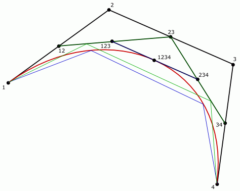Here the blue polyline is what we will have in case of adding point 1234, the green one is when adding points 23. It's obvious that the green line has less deviation. In practice it's 1.5…2 times less.

In the news group comp.graphics.algorithms I've got fair criticism for not being familiar enough with professional articles. The whole discussion is here. You can also find it in http://groups.google.com by key phrase “Adaptive Subdivision of Bezier Curves McSeem”.

One of the articles is called “Adaptive forward differencing for rendering curves and surfaces” and can be easily found in the Internet. The method described there is very nice, but it still doesn't solve the problem of smoothly looking strokes.

But the most interesting was a message from person with nickname Just d' FAQs. Here is the quotation:

A well-known flatness test is both cheaper and more reliable 
than the ones you have tried. The essential observation is that 
when the curve is a uniform speed straight line from end to end,
the control points are evenly spaced from beginning to end. 
Therefore, our measure of how far we deviate from that ideal 
uses distance of the middle controls, not from the line itself, 
but from their ideal *arrangement*. Point 2 should be halfway 
between points 1 and 3; point 3 should be halfway between points 
2 and 4.
This, too, can be improved. Yes, we can eliminate the square roots 
in the distance tests, retaining the Euclidean metric; but the 
taxicab metric is faster, and also safe. The length of displacement 
(x,y) in this metric is |x|+|y|.

In practice it means the following code.

    if(fabs(x1 + x3 - x2 - x2) +
       fabs(y1 + y3 - y2 - y2) +
       fabs(x2 + x4 - x3 - x3) +
       fabs(y2 + y4 - y3 - y3) <= m_distance_tolerance_manhattan)
    {
        m_points.add(point_type(x1234, y1234));
        return;
    }

It doesn't require forcing the first subdivision and it's absolutely robust in any case. The author insisted that this criterion is quite enough, but my additional experiments showed that the result is similar to what the incremental method produces. This estimation does not provide a good balance between the number of points and the approximation error. But it makes perfect sense to use it in all collinear cases. I have incorporated it and it seems that I can stop the research at this point. The method required different metrics, that is “Manhattan” (or “taxicab”), so that we will have to normalize the “tolerance” value like the following:

    m_distance_tolerance_square = 0.5 / m_approximation_scale;
    m_distance_tolerance_square *= m_distance_tolerance_square;
    m_distance_tolerance_manhattan = 4.0 / m_approximation_scale;

In all collinear cases it works better than the method Timothee Groleau suggested.

So, once again, the full source code is here: curve4_div, files agg_curves.h, agg_curves.cpp.